
Oliver Parish Machine Learning Engineer

John HughesAccuracy Team Lead
Integrating external language models (LMs) to automatic speech recognition (ASR) systems is widely used to increase accuracy while maintaining fast runtimes and low memory costs. Doing this allows you to benefit from billions of words collected from the internet rather than relying on the acoustic model to learn word relationships from transcripts alone (which is usually a few orders of magnitude less).
Recent end-to-end models such as the recurrent neural network transducer (RNNT) include an implicit internal language model (ILM) that is trained jointly with the rest of the network. This has the benefit of reducing the number of components that make up an ASR system and gives the ability to do greedy decoding with acceptable accuracy. However, it’s still very desirable to combine external LMs with RNNT models (often via shallow fusion) and it’s important to subtract the internal scores to get the best accuracy results.
In this blog, we will derive subtracting the LM scores stemming from Bayes’ rule and give a simple implementation of how it works in practise with K2’s streaming decoder. K2 is the next generation of Kaldi (a popular ASR framework) and it integrates FSTs into PyTorch. The recipes for running models can be found in Icefall and the dataset-related tools in Lhotse.
For conventional ASR models, you find the optimal word sequence (Ŵ) by doing maximum a posteriori decoding. This is when you find the word sequence (W) given the acoustic features (X) that maximizes the posterior. The posterior is given by Bayes’ rule:

When maximizing to find Ŵ, the probability of X is constant so drops out of the equation:

The acoustic model (AM) and the LM give you the likelihood P(X|W) and the prior P(W) respectively. A language model scaling factor (LMSF) denoted by λ₁ is often used since the AM tends to underestimate P(X|W) due to the independence assumption on phone probabilities. This factor can be tuned to recalibrate the trade-off between acoustics and common word sequences. The optimal path is now given by:

Taking the log of this function leads to:

During decoding the scores from the AM and LM are combined in a first pass that generates a lattice of possible word sequences by doing a beam search over possibilities. An n-gram LM is commonly used here due to being a quick lookup table. Following that there is a second pass where the arcs in the lattice are rescored by a neural LM. Finally, you search to find the optimal path (Ŵ) in the lattice. For more information on decoding and the LMSF see this blog.
When using the RNNT, how do we decode when the external LM and ILM both model P(W)? Let’s answer that next.
The RNNT is a popular end-to-end architecture used for ASR since it works in real-time unlike encoder-decoder architectures used by models like Whisper.
The RNNT model consists of 3 components, the encoder, the predictor, and the joiner which can be seen in the diagram below. The encoder takes acoustic data as inputs, the predictor takes the previously predicted tokens (word pieces / phonemes etc.) as input, and the joiner takes the output of the encoder and predictor and produces a probability distribution over tokens for each timestep. You can read a little more about sequence-to-sequence learning with transducers here.
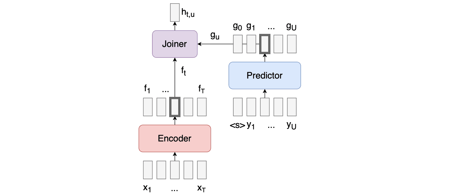
Since the predictor relies on previously predicted tokens to produce future token probabilities, it implicitly trains an ILM. Therefore, when using the RNNT you must be especially careful when integrating an external LM since there can be discord with the ILM due to being trained on different distributions of text. Google’s hybrid autoregressive transducer (HAT) was the first to integrate an external LM in a justified “Bayes way” by subtracting the ILM scores. But how do we arrive at that?
The RNNT directly models the posterior P(W|X) directly unlike the AM in conventional systems which models the likelihood P(X|W). Therefore, let’s use Bayes’ rule again, but this time to find the likelihood in terms of the RNNT posterior:

Since the ILM scores can only be estimated, let’s introduce another scale factor λ₂ and substitute this into Equation 3:

Finally, take the log:

This equation shows why applying Bayes’ rule leads to needing to subtract the ILM score. The intuition as to why this helps is that it removes the double contribution towards the text probability. This leads to over-reliance on the usual/likely word combinations in English and less on the actual acoustic data coming in. The weights λ₁ and λ₂ are tuned which can be a difficult balancing act to get right across many test sets. We’ll come back to tuning after looking at how we approximate the ILM.
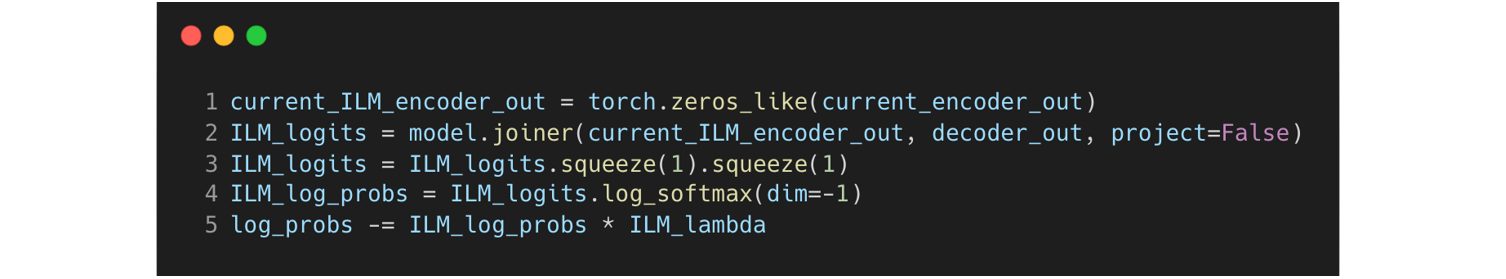
There are many ways to approximate the ILM. One fairly unintrusive way – and arguably the most effective – is to remove the contribution of the acoustic data by zeroing out the output of the encoder into the joiner. Another option which we have found not to be as effective is to take the average embedding over time or to model it with an LSTM as shown in this paper. This effectively allows the model to try to predict future tokens knowing nothing about the input acoustic data, making it a good proxy for the ILM.
You can easily integrate an external LM with K2’s fast_beam_search function implemented for the stateless RNNT. The following code zeros out the encoder and subtracts the ILM scores. This can be inserted before advancing the streaming decoder.
We use a 4-gram word piece language model and load it into a k2.fsa (see here). This is used during a beam search where the log probabilities we calculate above are repeated at each time step. Once this is complete you can create the lattice and find the best path through it. The log-probabilities of the external LM are added within K2’s decoder as shown in Equation 7 and the scale can be controlled (see here).
As we touched on earlier, to integrate the external LM effectively the two parameters λ₁ and λ₂ must be chosen carefully. These correspond to the external Language Model and Internal Language Model respectively.
Below are two sweeps over the parameter space, colored with the relevant word error rate (WER) reductions. Logically (and as can be seen in the plots), more ILM-subtraction introduces the need for more external LM addition to take up the slack.
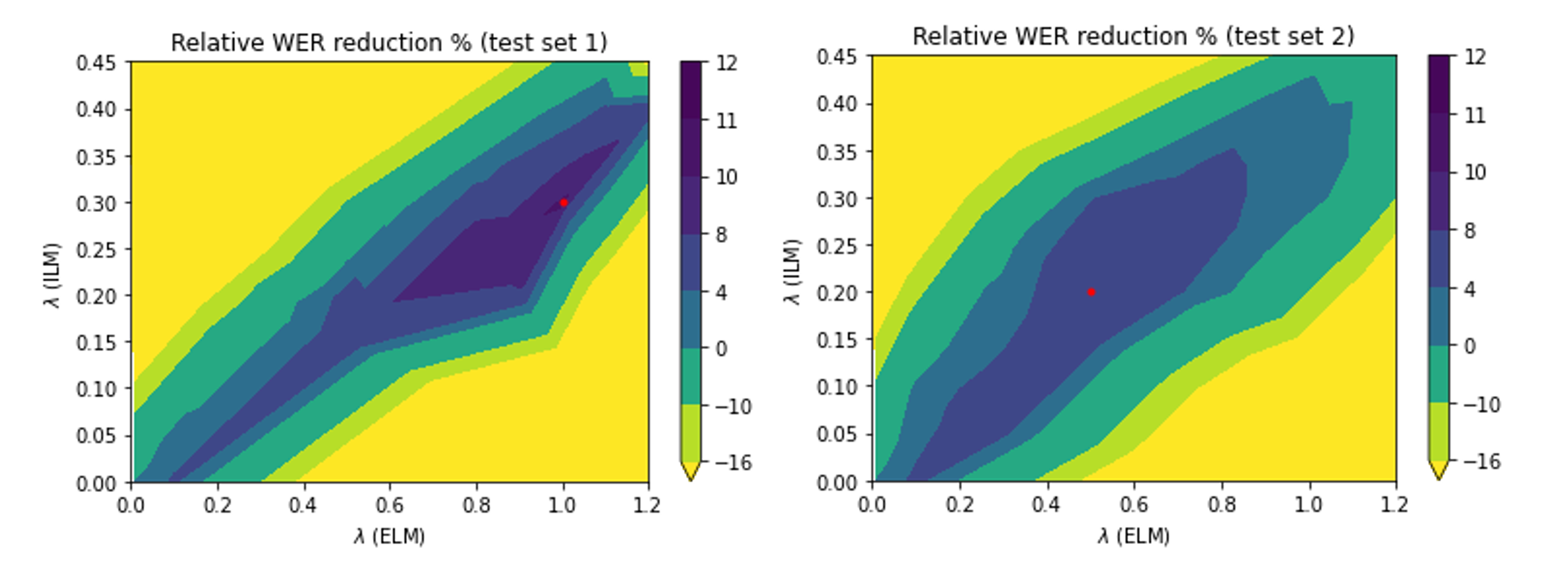
When sweeping over parameters, it also turns out that a key consideration is the dataset used. ILM parameters are sensitive to the dataset in question and the optimal choice may vary over different test datasets for the same model.
Above, the two sweeps refer to the same trained RNNT model over two different test sets. Though the profile of the two sweeps is similar, the optimal parameter choices differ substantially. This indicates that some thought needs to go into the choice of dataset to sweep. The set needs to encapsulate the data that the model will see in inference, otherwise parameter choice could lead to no improvements or even degradations.
If the choices are right, however, WER reductions can be found, in certain cases over 10% relative improvements are available.
One possible justification is that because the ILM is only trained on transcripts, the ILM can differ a lot in strength across test sets especially if they are out of domain. In other words, based on how similar the inference-time transcription is to the training transcripts, more or less ILM needs to be subtracted for optimal performance.
In conclusion, we can see the benefits of adding an external language model into an ASR system to boost accuracy quickly. However, when adding extra probability mass into the model predictions, it’s always important to think through exactly how these will interact with the original probabilities. As is often the way, balance is key.